Naive Bayes classifiers in TensorFlow

Naive Bayes classifiers deserve their place in Machine Learning 101 as one of the simplest and fastest algorithms for classification. This post explains a very straightforward implementation in TensorFlow that I created as part of a larger system. You can find the code here.

The textbook application of Naive Bayes (NB) classifiers is spam filtering, where word frequency counts are used to classify whether a given message is spam or not. In this example, however, we're going to be using continous data instead. More specifically, we'll be classifying flowers based on measurements of their petals size.

The algorithm

Just a quick refresher on the NB algorithm: as with any classifier, the training data is a set of training examples $\textbf{x}$, each of which is composed of $n$ features $\textrm{x}i = (x{1}, x_{2}, ..., x_{n})$ and their corresponding class $C_i$ where $i$ is one of $k$ classes. The goal is to learn a conditional probability model:

$$ p(C_k | x_1, x_2, ..., x_k) $$

for each of the $k$ classes in the dataset. Later, we're going to see how a simple rule can be used to make a decision on the basis of these conditional probabilities. Intuitively, learning this multivariate distribution will require a lot of data as the number of features grows. However, we can simplify the task if we assume that features are conditionally independent given the class. While this assumption never holds on real data, it results in a single but surprisingly simple classifier.

The math develops as follows. First, we write down Bayes' theorem:

$$ p(C_k | \mathbf{x}) = \frac{p_(C_k)p(\mathbf{x} | C_k)}{p(\mathbf{x})} $$

By definition of conditional probability, the numerator is just the joint probability distribution $p(C_k, \mathbf{x})$, and can be factored using the chain rule:

$$ p(C_k, \mathbf{x}) = p(x_1 | x_2, ..., x_n, C_k)p(x_2 | x_3, .., x_n, C_k)p(x_n | C_k)p(C_k) $$

By the naive assumption, the reciprocal conditioning among features can be dropped. In other words, we assume that the value assumed by each feature depends on the class only, and not on the values assumed by the other features. This means that we can simplify the previous formula quite a bit:

$$ p(C_k, \mathbf{x}) = p(x_1 | C_k)p(x_2 | C_k)...p(x_n | C_k)p(C_k) $$

Going back to Bayes' theorem, we observe that we can discard the denominator since it's just a normalization factor that doesn't depend on the class. We get:

$$ p(C_k | \mathbf{x}) \sim p(C_k, \mathbf{x}) \sim p(c_K)p(x_1|C_k)p(x_2|C_k)p(x_3|C_k) \sim p(C_k)\prod_{i=1}^{n}p(x_i | C_k) $$

The last formula shows why NB is so convenient: all $p(x_i | C_k)$ distributions can be learned independently. During training, we can split the examples by label, then learn a univariate distribution for each of the features given the class. For this example, we're going to assume that $p(x_i | C_k)$ are Gaussian distributions whose $\mu$ and $\sigma$ we can estimate easily from the samples.

To wrap up the algorithm, we need to make a decision based on these conditional probabilities. An intuitive and very common strategy is **Maximum a Posteriori (MAP)*: we simply pick the most likely class:

$$ \underset{k \in {1,..,K}}{\arg\max}\ p(C_k) \prod_{i=1}^np(x_i | C_k) $$

The scikit baseline

With sklearn, loading the dataset and training the classifier is trivial:

from sklearn.naive_bayes import GaussianNB
gnb = GaussianNB()
gnb.fit(X, y)

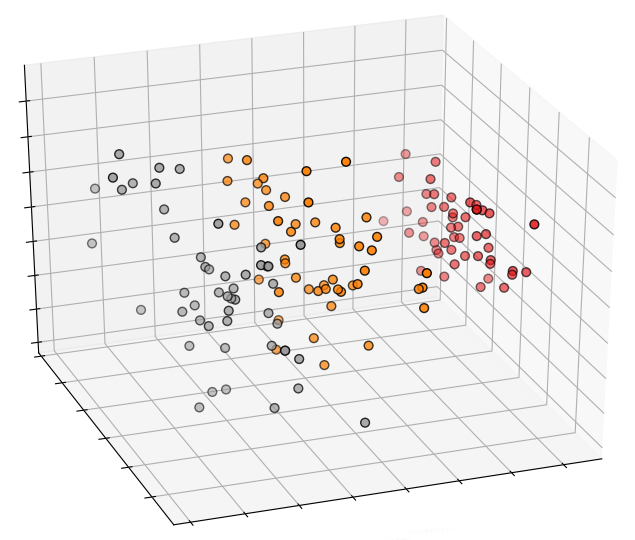
This is how a plot of the 3 first principal components looks like in 3D:

TensorFlow implementation

You may want to follow along with the actual code here.

Training

We start by grouping the training samples based on their labeled class, and get a (nb_classes * nb_samples * nb_features) array.

Based on the discussion above, we can fit individual Gaussian distributions to each combination of labeled class and feature. It's important to point out that, even if we're feeding the data in one go, we are fitting a series of univariate distributions, rather than a multivariate one:

mean, var = tf.nn.moments(tf.constant(points_by_class), axes=[1])

In this trivial example, we're using tf.constant to get the training data inside the TensorFlow graph. In real life, you probably want to use tf.placeholder or even more performing alternatives like tf.Data (see the documentation).

We take advantage of TensorFlow's tf.distributions module to create a Gaussian distribution with the estimated mean and variance:

self.dist = tf.distributions.Normal(loc=mean, scale=tf.sqrt(var))

This distribution is the only thing we need to keep around for inference, and it's luckily pretty compact, since the mean and variance are only (nb_classes, nb_features).

Inference

For inference, it's important to work in the log probability space to avoid numerical errors due to repeated multiplication of small probabilities. We have:

$$ \log p(C_k | \mathbf{x}) = \log p(C_k) + \sum_{i=1}^n \log p(\mathbf{x} | C_k) $$

To take care of the first term, we can assume that all classes are equally likely (i.e. uniform prior):

priors = np.log(np.array([1. / nb_classes] * nb_classes))

To compute the sum in the second term, we duplicate (tile) the feature vectors along a new "class" dimension, so that we can get probabilities from the distribution in a single run:

# (nb_samples, nb_classes, nb_features)
all_log_probs = self.dist.log_prob(
    tf.reshape(
        tf.tile(X, [1, nb_classes]), [-1, nb_classes, nb_features]))

The next step is to add up the contributions of each feature to the likelihood of each class. In TensorFlow lingo, this is a reduce operation over the features axis:

# (nb_samples, nb_classes)
cond_probs = tf.reduce_sum(all_log_probs, axis=2)

We can then add up the priors and the conditional probabilities to get the posterior distribution of the class label given the features:

joint_likelihood = tf.add(priors, cond_probs)

In the derivation, we ignored the normalization factor, so the expression above is not a proper probability distribution because it doesn't add up to 1. We fix that by subtracting a normalization factor in log space using TensorFlow's reduce_logsumexp. Naively computing log(sum(exp(..))) here won't work here because of numerical issues (see the logsumexp trick).

norm_factor = tf.reduce_logsumexp(
    joint_likelihood, axis=1, keep_dims=True)
log_prob = joint_likelihood - norm_factor

Finally, we exponentiate to get actual probabilities:

probs = tf.exp(log_prob)

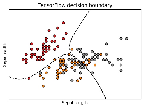
By feeding in a grid of points and drawing the contour lines at 0.5 probability, we get the nice plot at the top:

Conclusion

Building a simple Naive Bayes classifier in TensorFlow is a good learning exercise to get familiar with TensorFlow's probability distributions and practice the less common tensor operations.