SLAM loop closure with TensorFlow

Having looked at a simple implementation of SLAM loop closure detection using "conventional" algorithms, I wanted to try replacing hand-rolled features with those learned by a CNN.

In this article, we are going to use TensorFlow and its pre-trained Inception v3 network to try to detect previously-visited places within the New College image dataset (available here). I've picked the Inception model since its weights are relatively compact (~ 50 MB) and the final pooling layers have just about the right dimensions for a compact representation of the frame. Since the model weights were trained on the ubiquitous ImageNet dataset, this is going to be an exploration of transfer learning.

However, this application is rather exotic and likely a bad match for common CNNs originally architected for image classification. In particolar, the pooling layers discard a lot of the spatial relationships that would be useful for loop detection. For now, let's look at what we can get out of a standard model.

Setting up the model

The pre-trained inception model is available for download from the TensorFlow site.

We can easily load its graph definition:

import os
import json
from glob import glob

import numpy as np
import seaborn as sns
import scipy.io as sio
import tensorflow as tf
import matplotlib.pyplot as plt
from tensorflow.python.platform import gfile

%matplotlib inline

with gfile.GFile('classify_image_graph_def.pb', 'rb') as f:
    graph_def = tf.GraphDef()
    graph_def.ParseFromString(f.read())

TensorFlow makes extracting intermediate representations pretty easy: we can request a specific tensor using the Graph.get_tensor_by_name function. This pre-trained model also nicely handles arbitrarily-sized JPEGs, so that we don't have any preprocessing to do.

def forward_pass(fname, target_layer='inception/pool_3:0'):
    g = tf.Graph()

    image_data = tf.gfile.FastGFile(fname, 'rb').read()

    with tf.Session(graph=g) as sess:
        tf.import_graph_def(graph_def, name='inception')

        pool3 = sess.graph.get_tensor_by_name(target_layer)
        pool3 = sess.run(pool3,
                         {'inception/DecodeJpeg/contents:0': image_data})

        return pool3.flatten()

Let's try running the forward pass on a sample image:

from IPython.display import Image
Image(filename='ferrari.jpg', width=300)

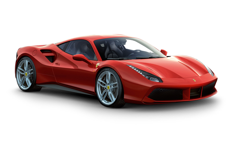
ferrari_repr = forward_pass('ferrari.jpg')
ferrari_repr
array([ 0.26067936,  0.2310448 ,  0.48140237, ...,  0.33839288,
        0.51758009,  0.04004376], dtype=float32)

At this stage in the CNN, the representation is already pretty compact:

ferrari_repr.shape
(2048,)

Processing the dataset

We can now easily run through all the images in the dataset and extract their 2048-element representations:

# Use [::2] to keep images from the left camera only
filenames = sorted(glob('/home/niko/NewCollege/*.jpg'))[::2]

representations = []

for fname in filenames:
    frame_repr = forward_pass(fname)
    representations.append(frame_repr.flatten())

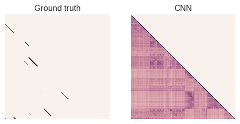
As discussed in my previous article, we can plot the confusion matrix to visualize the estimated similarity between any two frames in the dataset.

In this case, I'm going to use the $L_2$ metric to score the distance between the representation vectors.

def normalize(x): return x / np.linalg.norm(x)

def build_confusion_matrix():
    n_frames = len(representations)

    confusion_matrix = np.zeros((n_frames, n_frames))

    for i in range(n_frames):
        for j in range(n_frames):
            confusion_matrix[i][j] = 1.0 - np.sqrt(
                1.0 - np.dot(normalize(representations[i]), normalize(representations[j])))

    return confusion_matrix

confusion_matrix = build_confusion_matrix()

# Load the ground truth

GROUND_TRUTH_PATH = os.path.expanduser(
    '~/bags/IJRR_2008_Dataset/Data/NewCollege/masks/NewCollegeGroundTruth.mat')

gt_data = sio.loadmat(GROUND_TRUTH_PATH)['truth'][::2, ::2]

# Set up plotting

default_heatmap_kwargs = dict(
    xticklabels=False,
    yticklabels=False,
    square=True,
    cbar=False,)

fig, (ax1, ax2) = plt.subplots(ncols=2)

# Plot ground truth
sns.heatmap(gt_data,
    ax=ax1,
    **default_heatmap_kwargs)
ax1.set_title('Ground truth')

# Only look at the lower triangle
confusion_matrix = np.tril(confusion_matrix, 0)

sns.heatmap(confusion_matrix,
           ax=ax2,
           **default_heatmap_kwargs)
ax2.set_title('CNN')

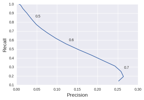
Precision-recall performance

Looking at the precision-recall curve I explained in the previous article gives a more objective measure of performance. For the sake of simplicity, let's use a thresholding operation to classify loop closures. We can then build the PR curve by a simple sweep of the threshold parameter, as done in the following block of code:

prec_recall_curve = []

for thresh in np.arange(0, 0.75, 0.02):
    # precision: fraction of retrieved instances that are relevant
    # recall: fraction of relevant instances that are retrieved
    true_positives = (confusion_matrix > thresh) & (gt_data == 1)
    all_positives = (confusion_matrix > thresh)

    try:
        precision = float(np.sum(true_positives)) / np.sum(all_positives)
        recall = float(np.sum(true_positives)) / np.sum(gt_data == 1)

        prec_recall_curve.append([thresh, precision, recall])
    except:
        break

prec_recall_curve = np.array(prec_recall_curve)

plt.plot(prec_recall_curve[:, 1], prec_recall_curve[:, 2])

for thresh, prec, rec in prec_recall_curve[25::5]:
    plt.annotate(
        str(thresh),
        xy=(prec, rec),
        xytext=(8, 8),
        textcoords='offset points')

plt.xlabel('Precision', fontsize=14)
plt.ylabel('Recall', fontsize=14)

Comments and future work

As it stands, this deep-learning representation works rather poorly for our purposes. My intuition is that, as CNN architectures get more and more optimized for classification, their performance on other tasks decreases. Also, the ImageNet dataset that was used for training looks nothing like the drab British countryside in the localization test.

---