Car speed estimation from a windshield camera

Measuring the speed of car by capturing images from a windshield camera is a seemingly easy computer vision problem that actually isn't.

That's because geometry is unforgiving, and a single camera lacks the sense of depth needed to estimate speed without any assumption about the environment. It just so happens that humans subconsciously use higher-level visual clues that help them disambiguate the absolute scale of the scene (i.e. road lanes are a few metres across).

This post is going to explore a few potential solutions.

A few alternatives

One idea would be to leverage decades of research in monocular odometry and SLAM, and use an open-source package from any research group worldwide. I have benchmarked a few of those in a previous post. Semi-direct Visual Odometry (SVO), which I hadn't mentioned in the article, could also be a good match for this problem.

While all of these approaches start out by detecting interest points across the image, they differ in the way the recover the camera motion. SLAM packages, such as ORB or Rovio, explicitly estimate scene structure in the form of a sparse map of landmarks whose location is found incrementally. Instead, visual odometry uses concepts from projective geometry, such as the essential matrix, to estimate the camera motion from feature matches alone.

All of these techniques solve a much more general problem than the one we have at hand. Not only do they estimate camera velocity, but also its position and 3D orientation. Such power and generality comes at the cost of increased need for calibration.

Ideally, we would only need to calibrate the system once (when it's installed in the car), and not every time we start a new trip.

This requirement rules out any of the monocular SLAM/odometry systems, since their calibration also depends on the scene structure, which is different for each trip. In other words, the sight of an object on a single camera doesn't provide any absolute speed information, since its apparent motion in the frame depends on its distance as well as the camera motion. Using a single camera it's not possible to disambiguate between these two factors.

Since none of these powerful ideas lends very well to our problem, we're going to turn to a simpler approach that's easier to specialize for our current task.

Taking the simple(r) approach

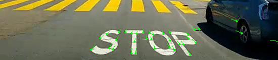
Optical flow is one of the most basic concepts in computer vision, and refers to the apparent motion of objects in the image due to the relative motion between the camera and the scene. When optical flow is computed for individual features across the frame, it shows up as vectors that are tangent to the apparent motion of the feature in the frame. Here's an example:

Monocular optical flow suffers from the same ambiguity problems that we discussed above, and is thus not enough to estimate metric speed. We'll need to make more assumptions about the structure of the scene.

Following the approach in [@Giachetti1999], we assume that the car is traveling over a flat road that can be modeled as a plane. In this particular case, the two components $u, v$ of the optical flow at point $(x, y)$ are a quadratic function of the coordinates themselves:

$$ u = c_{13}x^2 + c_{23}xy + (c_{33} - c_{11})fx - c_{21}fy - c_{31}f^2 $$ $$ v = c_{13}xy + c_{23}y^2 + (c_{33} - c_{22})fy - c_{12}fx - c_{32}f^2 $$

where $f$ is the focal length of the camera.

We can further simplify these equations by assuming that the road plane is orthogonal to the camera plane and parallel to its velocity. Both of these requirements are reasonable in our context. The simplified equations can be written as:

$$ u = \frac{\omega}{f}x^2 + \frac{V}{hf}xy + \omega f $$ $$ v = \frac{\omega}{f}xy + \frac{V}{hf}y^2 $$

where $V$ and $\omega$ are the linear and angular velocities of the camera, and $h$ is the distance between the camera and the plane (i.e. road).

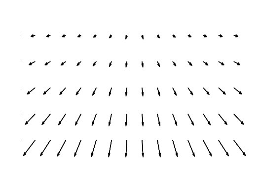
Given the sort of test data that I had available, it made sense to discard the rotational term and only consider the optical flow induced by the translational velocity. In hindsight, this made sense as errors in the flow estimation vastly outweighted the small contributions due to camera rotations. That's how the resulting flow looks like in theory:

Under this final assumption, we only need ground-truth data to calibrate the $hf$ factor, which incorporates the effect of the focal length of the camera and its height over ground.

Implementation

I implemented the tracking and estimation code using OpenCV for the sparse optical flow function, and a few Numpy functions for the least squares fitting. It's less than 200 lines that you can find here.

Due to the assumptions we made when building the model, it's very important to make sure that we're only looking at the optical flow on road points. Some rough cropping and masking almost sort-of partially worked on the dataset I had. A more robust system would use a real image segmentation algorithm to filter out the road points. Here's an example of the map I've used:

The top rectangle blocks out detection in areas where other cars are likely to appear, while the area on the right improves estimation quality by discarding the flow from buildings and other disturbances.

Results and sticking points

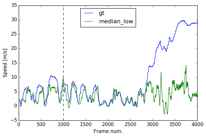
I used the optical flows from the first 1000 frames together with the ground truth to fit the $hf$ factor using least squares. The speed on the following frames can be then estimated as shown above.

I've tried both mean and median to get rid of noise when going from hundreds of flow measurements to a single value for the vehicle speed. I've also done some rough low-passing on the resulting value to smooth out the speed over time (as expected for a real vehicle).

As you can see below, the results are decent at low speeds, but deteriorate quite a lot at highway speeds. That's probably due to very bad optical flow tracking on the highway images, on which very few features were tracked at all.

I should also implement outlier rejection for the flow vectors, as that should reduce noise and allow reducing the strength of the low-pass filter to speed up the dynamic response. Some more improvement ideas are described in [@Barbosa2007].

Again, the code for this lives on Github.

---