Robotics for developers 6/6: adding an accelerometer

In a previous post we added multiple camera states to track the robot's movement over time. In that configuration, however, localization data is only available when a marker is captured by the camera. In this post, we'll see how adding a new sensor source can help the system localize the robot for brief periods of time even when no marker is visible.

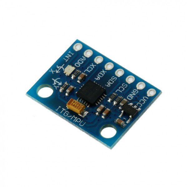
An inertial measurement unit (IMUs) is a mechanical device that can measure its acceleration and angular velocity. By mounting one of these sensors on a robot, the SLAM system gains valuable information about motion, that can be used to improve localization accuracy.

While there are several kinds of IMUs on the market, most robotic applications use so-called MEMS IMUs, due to their small size and limited weight. These devices include two different components: an accelerometer (to measure acceleration) and a gyroscope (to measure angular velocity).

Unfortunately, IMUs can not be used directly for navigation, since they don't measure position or orientation, but rather their time derivatives (second derivative in the case of the accelerometer, and first in the case of the gyroscope). Calculus tells us that we would need to integrate the sensor data to compute the robot position and orientation. However, this operation is strongly sensitive to noise, since any small error in the derivatives will grow unbounded over time. In real applications, such sensitivity shows up as divergence of the localization estimate. That's the reason why drones constantly require GPS reception or cameras to stabilize themselves, as the onboard sensors are useless after 20-30 seconds.

It turns out that not all hope is lost. IMUs and vision data are nicely complementary sources. IMUs offer much higher data rate (~200Hz vs ~20Hz) but drift over time. Processing image data requires more processing power than integrating the IMU measurements, but can stabilize the system over time.

For these reasons, we will be integrating IMU measurements into the SLAM optimization implemented in the previous posts. We'll see how the IMU can provide reasonably good location estimates even when no markers are visible in the camera frame for brief periods (~5 seconds). Furthermore, the IMU will also allow us to reduce the camera frame rate (and thus the processing load) while retaining access to a high-frequency navigation-solution.

Adding IMUs to the localization problem

Using IMUs for SLAM is quite involved, since many of the measurements and states and correlated by a non-trivial measurement model. Luckily, GTSAM comes with a powerful factor to handle sensor data from an IMU, implemented according to this paper. Due to Physics, the IMU factor is slightly more involved than the other factors we have used.

Until now, the estimation has only concerned the camera frame, that we identified with the robot position in the world. However, now that we introduced an IMU as well, we'll need to distinguish between a camera frame (that observes the marker) and the body frame (location of the IMU). The transformation between these two frames can either be measured beforehand using a ruler, calibrated offline, or estimated online as part of the localization process. We'll be using the second approach, since the datasets already come with the calibration data.

From the estimation point of view, the IMU factor constrains successive positions and orientations in time. The gyroscope directly measures angular velocity, so that it can directly be used to constrain two successive orientation states (the math is a bit hairy though, as it uses incremental rotations). The acceleration as measured by the accelerometer, however, can not be used directly, since it's the second derivative. To handle this, we also need to keep the velocity of the robot as part of the estimation states.

We need one final change, due to the way that accelerometers and gyroscope work. In real life, their measurements are not exact, but are biased. This can be modeled by adding a pair 3-dimensional bias terms to the measurement models of the IMU. The bias will be different each time the sensor is turned on, so it can not easily be calibrated out, but will change rather slowly over time. This means we can easily estimate the two biases as part of the estimation process.

To recap, the IMU factor will be connected to a variety of states: the previous and current poses (position + orientation), the current pair of biases, and the current and previous velocities. That's how it looks like in code:

    graph_.add(
    	gtsam::ImuFactor(s_prev_ic, s_prev_vel,
    					 s_ic, s_vel, s_bias,
    					 pre_integr_data));

Note that the implementation in GTSAM has the concept of IMU preintegration, i.e. accumulates a packet of measurements and adds multiple ones in a single factor (the paper linked above has more details). This reduces the size of the graph and thus the computational load, since we can keep adding pose states at camera frame rate, rather than the much higher IMU rate.

As explained above, the pair of biases is modeled as a random walk, and we thus also need to add a simple BetweenFactor to model their time evolution. Following the concept of a random walk, we expect the change in biases to be zero. The noise model for this factor depends on the quality of the sensor and can be calibrated or extracted from its datasheet.

auto bias_between_noise = gtsam::noiseModel::Diagonal::Sigmas(
        sqrt(pre_integr_data.deltaTij()) * bias_between_sigmas_vec_);

graph_.add(
        gtsam::BetweenFactor<gtsam::imuBias::ConstantBias>(
        s_prev_bias, s_bias,
        gtsam::imuBias::ConstantBias(), bias_between_noise);

Gravity and initial calibration

One detail I've glossed over above is the initialization of an IMU-based system. Since the sensing elements of accelerometers are subject to gravitational acceleration (just like any other body on the surface of Earth), the values they measure include a gravitational acceleration term.

Obviously, this term must be accounted for in the measurement model. According to ROS conventions, we use a navigation frame with upwards Z axis, and inform the factor of such:

preint_params_ = gtsam::PreintegrationParams::MakeSharedU(9.81);

To make sure that the system works properly, it's important that the initial body orientation is coherent with the gravity direction. In most applications, it can be safely be assumed that the robot is initially stationary. Under this assumption of zero motion, the accelerometer only measures gravitational acceleration. This means that a good estimate of the initial orientation can be found by requiring that the measured gravity vector transformed to the world frame through the initial pose matches the upwards direction. That's what we do in the do_accel_init function:

void do_accel_init() {
    gtsam::Vector3 acc_avg;
    for (auto &kv : imu_meas_) {
        acc_avg += kv.second.first;
    }
    acc_avg /= imu_meas_.size();
    ROS_WARN_STREAM("Gravity-aligning with accel. vector:\n" << acc_avg);

    gtsam::Vector3 gravity_vec;
    gravity_vec << 0.0, 0.0, gravity_magn_;
    auto initial_att = gtsam::Rot3(
    	Eigen::Quaterniond().setFromTwoVectors(acc_avg, gravity_vec));
    initial_pose_ = gtsam::Pose3(initial_att, gtsam::Point3());

    (initial_pose_ * acc_avg).print("Gravity vector after alignment:\n");

    accel_init_done_ = true;
}

Localization without markers

To show that the IMU really improves performance, we can artificially disable marker tracking for a few seconds and compare the pose predicted using the IMU to the one computed by marker tracking. This trick simulates a tracking failure and will ensure that the biases have converged and that the coordinate transformations are correct.

The following plots compare the prediction to the final estimate after optimization. You can see how the two tracks of values are pretty close, since the fiducial marker is tracked at 20Hz and the IMU measurements don't have time to diverge. The section without data points in the middle is the artificial pause.

The most important point is the one right after marker tracking resumes. You can see how the gyroscopes are incredibily accurate, and the rotation estimate agrees almost perfectly with the vision estimate. Accelerometers are less precise, but their estimate is still good.

Bias estimation

As mentioned above, correct modeling of IMU errors requires online estimation of accelerometer and gyroscope biases. To double-check that everything is working correctly, we look at the evolution of one component of the bias over time:

The bias hovers around a very small value, showing that the constraints from the markers are enough to estimate it. This fact is part of the broader topic of observability analysis, which analyzes which states of a system can be observed given a certain set of sensors.

Conclusions

We have seen how adding an IMU can make the SLAM system more robust to missing visual information and potentially reduce the computational load. Since these sensors are cheap and light, they're now a staple of state estimation in drones and all sort of gadgets, including Google Tango.