Robotics for developers 3/6: using the camera

The previous post showed how to use probability theory and non-linear optimization to integrate different sources of information. But what kind of data does the observation of a fiducial marker actually produce? How can we find out the position of the camera with respect to the marker once we know its size and position within the image? In other words, what's the form of the measurement factor that gets added to the factor graph?

The pinhole model

We're going to use concepts from geometric computer vision to exploit the relationship between the position of the marker corners in the captured image and in the real world. To do this, we need to introduce a model for the physical behavior of a digital camera. While things can generally get hairy here, it's enough to say that a camera projects 3D points in the environment to 2D points in the sensor plane. ¹ Some basic geometry helps here, as shown in the following image (the dotted frame is the sensor plane):

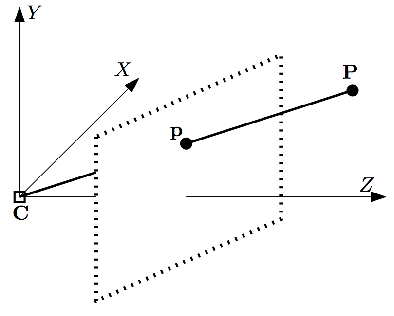
The picture represents the relationship between world point $P$ (world_p 3-vector), and image point $p$, (image_p 2-vector). There's a straightforward mathematical relationship between $P$ and $p$, that can be expressed as: ²

image_p[0] = world_p[0] * f_x / world_p[2] + o_x
image_p[1] = world_p[1] * f_y / world_p[2] + o_y

As you will have noticed, there are three unknown parameters in the equation: f_x, f_y, o_x, o_y. These numbers are intrinsic properties of the imaging system (camera + lens combination) and are the same for any point in any frame. They're usually obtained through the process of intrinsic calibration of the camera, which we're going to happily skip, since it's well-covered online and doesn't require much insight. There's a bit more on this topic, namely introducing corrections for lens imperfections, but it's not very important for a full understanding.

In mathematical terms, the pinhole projection equations can be written as:

Reprojection error

Thanks to the previous two sections, we have all the building blocks needed to write down the measurement model for a single point. Given a measurement (in our case, the position of a corner in a captured image), and the current estimate of the camera position (the state), the measurement model will tell the optimizer:

• how well the current estimated state agrees with the measurement,
• the direction in which to "wiggle" the estimated state to improve such agreement ³

To make things simpler, we can assume that the camera is at position $(0, 0, 0)$. Later, we'll see how it's generally more convenient to have one of the markers in this position, and leave the camera floating in space.

In any case, given that we know the position of the camera, the situation is just like the projection picture above, and the state will simply be the position of the corner point in the world.

The pinhole equations, expressed here by the function project, are all we need to write the measurement model: ⁴

error[0] = measured_image_p[0] - project(world_p)[0]
error[1] = measured_image_p[1] - project(world_p)[1]

The equations above compute the reprojection error for a single point correspondence. The array notation emphasizes that the reprojection error is a two dimensional vector (one horizontal and one vertical term). Note how the vector dimensions all match: project takes a 3D points and returns a 2D point, just like measured_image_p is.

In our case, we need to consider multiple points at the same time (at least 4). There's nothing preventing us from extending the error vector above with additional point correspondences. However, the next section will explain why this is a bad idea.

What about the other corners?

The problem with having a 8-vector error for each marker (4 corners * 2 points per corner) is that each corner would be optimized independently. This is not correct though since the position of each is related to the others (as they're all part of the same rigid object - the marker).

The way we solve this is by adopting a better definition of the state. Instead of having the position of points, we're going to optimize over the marker pose. Note that I've wrote pose, not position. Since the marker is a whole object, not just a single point, we need to define its orientation as well as its position.

While the basic concept is straightforward (define a set of rotations to align the marker with some reference, such as a floor tile), rotation representations are a dime a dozen and wildly confusing. Luckily, we're going to take advantage of classes and functions offered by the GTSAM framework to tackle most of this issues. ⁵

Instead, let's focus on using this new state to write the right reprojection error for a whole marker. We can look at the marker pose as the position of the center point of the marker, together with the orientation of its frame of reference. To compute the position of each of the 4 corner points, we just need to compose the marker pose with vectors going from the center of the marker (our reference point) to each of them. Luckily, these vectors are easy to compute, since we know the side length of the marker (we just need to pay some attention to the signs and directions). The figure below shows a 2D simplification of the concept:

While there's much more mathematics behind this, we can use the power of software abstraction and ignore most of it. Indeed, most optimization frameworks make it easy to abstract away rotations and translations without caring about the underlying representation.

Leveraging an existing marker detector and datasets

As mentioned in the previous post, we're going to be taking advantage of datasets provided by the community instead of setting up our own hardware platform. This also means that we're going to have to choose the same marker detector they did.

For this project, I've picked datasets from the RCARS project by ETH Zurich, since they are recorded with a nice stereo camera and include ground truth and accelerometer data that will be useful as we progress in the project. For reference, that's how the images look like:

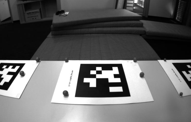
Since the marker detector they used doesn't compile on Ubuntu 16.04, I've decided to cheat, ran the detection on a different machine, and recorded the results in a new file. This also makes for a smaller download, since we won't need the images anymore, but just the position of the corners and their ids. ⁶

Let's take one of these datasets and examine it with rosbag info:

types:       geometry_msgs/TransformStamped [b5764a33bfeb3588febc2682852579b0]
             rcars_detector/TagArray        [f8c7f4812d2c3fcc55ab560a8de1d680]
             sensor_msgs/CameraInfo         [c9a58c1b0b154e0e6da7578cb991d214]
             sensor_msgs/Imu                [6a62c6daae103f4ff57a132d6f95cec2]
topics:      /cam0/camera_info       1269 msgs    : sensor_msgs/CameraInfo
             /imu0                  12690 msgs    : sensor_msgs/Imu
             /rcars/detector/tags    1269 msgs    : rcars_detector/TagArray
             /vicon/auk/auk          6343 msgs    : geometry_msgs/TransformStamped

For now, all the data we need to feed into the optimizer is in the /rcars/detector/tags and /cam0/camera_info (that contains the intrinsics parameters as described above).

Putting everything together - code!

What follows is a walk-through of the code I've pushed here. We're going to gloss over most of the boring sections and focus on the juicy parts, as it's easy to pick up the former from examples and ROS tutorials. ⁷

To start, we setup containers for the problem structure and the values associated with each element of the state:

gtsam::NonlinearFactorGraph graph;
gtsam::Values estimate;

Each piece of the state needs a label (gtsam::Symbol) that will identify it during the optimization problem. We create one for the camera pose and one for the marker pose:

auto s_camera = gtsam::Symbol('C', 0);
auto s_marker = gtsam::Symbol('M', 0);

The optimization needs to start somewhere, so we pick initial guesses and insert them in the Values container:

estimate.insert(s_marker, gtsam::Pose3());
auto cam_guess = gtsam::Pose3(gtsam::Rot3(), gtsam::Point3(0, 0, 0.5));
estimate.insert(s_camera, cam_guess);

In this example, the initial guess for the camera pose is 0.5 meters away from the marker, in the $z$ direction. As with any nonlinear optimization problem, the initial guesses should be chosen quite carefully, otherwise the optimizer may fail. This has been the subject of many a PhD's theses, so we won't cover it here.

The next step is picking a reasonable noise model to encode our degree of trust on the measurements. We're going to be using Gaussian distributions here since the marker detection is pretty robust and unlikely to produce outliers (hopelessly wrong values, as opposed to slightly incorrect measurements due to normal errors). Robust handling of outliers is another can of worms which is usually taken care of using robust estimators.

auto pixel_noise = gtsam::noiseModel::Isotropic::shared_ptr(
	gtsam::noiseModel::Isotropic::Sigma(8, 1));

The standard deviation of 1 pixel is pretty common in practice. It's now time to create a prior factor to encode our belief that the marker pose is close to the identity. The way this works is that I've decided that I want the marker to be in the origin pose, and thus create the prior accordingly. I could have set this prior anywhere (for example, 5 meters east), with no changes. However, a prior is indeed required otherwise the information in the measurement would not be enough to constrain the camera pose. This is somewhat intuitive, since it's clear that observing an object at a certain distance doesn't tell us where the camera is at all. That's why we need to add this additional belief.

auto origin_noise = gtsam::noiseModel::Isotropic::shared_ptr(
	gtsam::noiseModel::Isotropic::Sigma(6, 1e-3));

graph.push_back(
  gtsam::PriorFactor<gtsam::Pose3>(s_marker, gtsam::Pose3(), origin_noise));

It's finally time to add the measurement corresponding to the marker observation. We do this with the MarkerFactor class that embeds the reprojection error calculation:

graph.push_back(
  MarkerFactor(corners, pixel_noise, s_camera, s_marker, K_, tag_size_));

This factor is more complicated than the others, since it must be connected to both the marker and the camera poses and also needs the camera calibration (K_) and the side length of the marker (tag_size_).

Now that the factor graph is set up, we can kick off the optimization and relax:

auto result = gtsam::GaussNewtonOptimizer(graph, estimate).optimize();
auto opt_camera_pose = result.at<gtsam::Pose3>(s_camera);

The choice of the optimization algorithm has a significant effect on the convergence properties, speed and accuracy of the solution. Since the problem here is pretty straightforward, a basic textbook choice like Gauss-Newton's is fine.

Comparison with OpenCV

Our current approach is definitely overkill for such a simple measurement, and indeed OpenCV provides a built-in function to replace it all. Indeed, the solvePnP function will solve the 2D->3D scene reconstruction problem in the exact same way as we did.

We compare its results with our solution by plotting one coordinate of the camera position over time:

The numbers are so close that you actually need to hover to see both. You can also see a brief hole in the plot, corresponding to a few moments in which the markers was outside the frame.

Next steps

Now that we've set up the plumbing and checked that our computer vision fundamentals are sound, we can quickly iterate to make the project more useful, starting with tracking the robot as its camera moves over time. This is the subject of the next post in the series.

Notes